Non rigid diffusion: Application to shape matching

Objective: data-driven shape matching

Final objective: shape matching

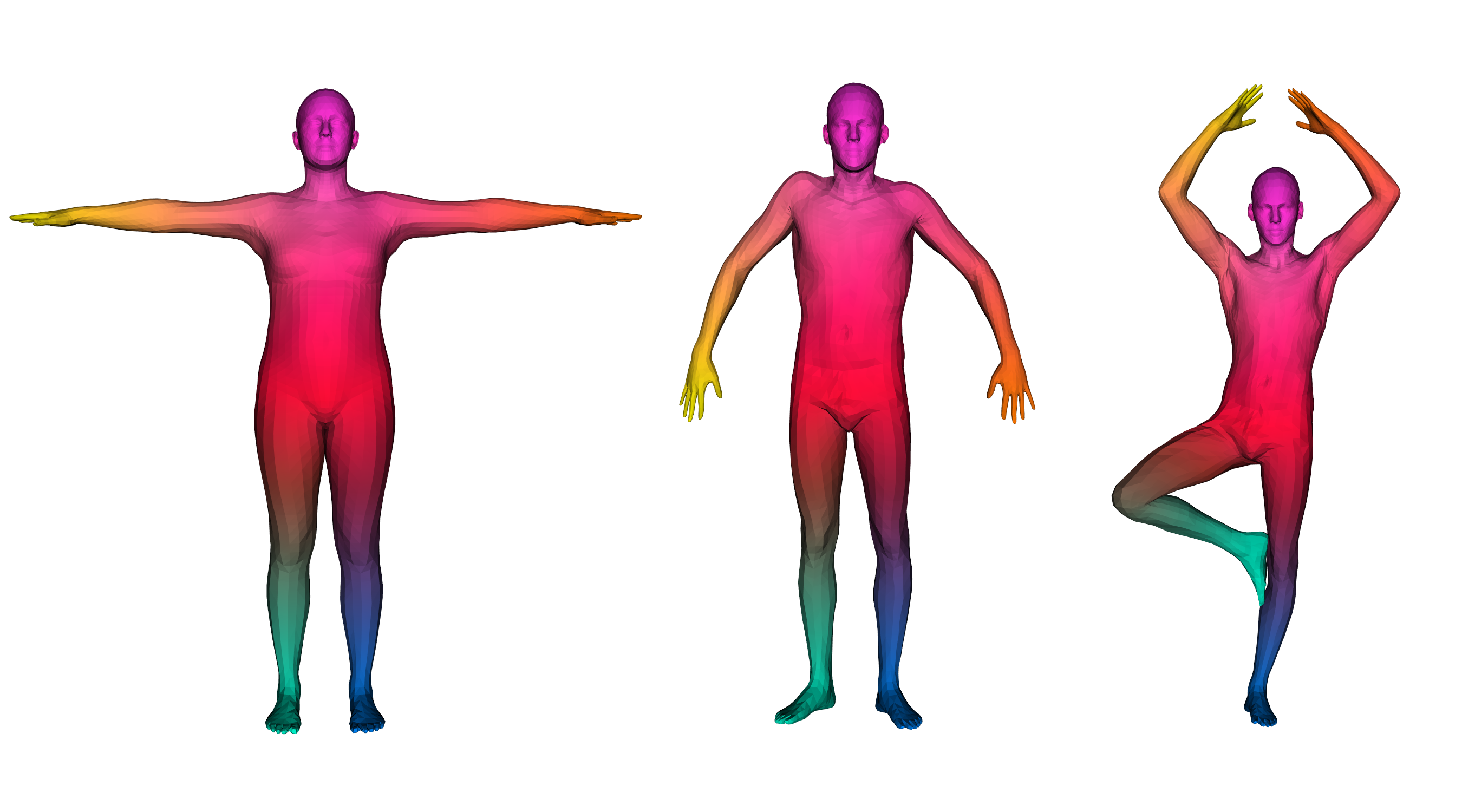
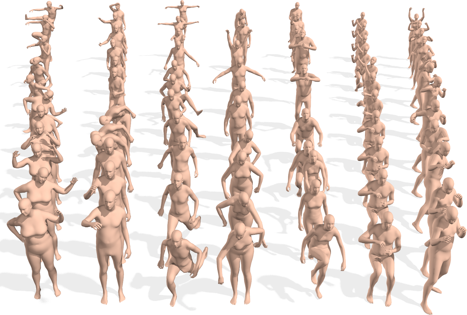
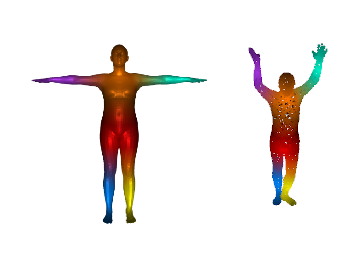
Vizualization of a point-to-point map between a template and 2 human shapes

We have access to huge datasets of non rigid shapes nowadays.

A few shapes of AMASS. The whole dataset contains around 100 million poses

The objective is to take profit of some huge databases of non rigid shapes to improve shape matching algorithms.

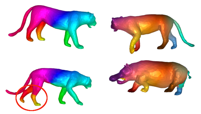
Shape matching algorithms are not perfect

A general problem in non rigid shape matching is dealing with symmetries. Regularizing algorithms with axiomatic constraints are not sufficient to get rid of this problem.

Example of a map where some parts of the arms are switched because of the natural symmetry of the human body. In gray, the template shape, in pink the target shape and in blue the target shape with connectivity transferred from the template shape via functional maps extracted using Lei’s approach

Is there a data-driven way to regularize the functional map and solve this problem ?

Background: Functional maps

Let \(M\), \(N\) two shapes. We aim to find a pointwise map \(T : M \to N\)

The idea is to represent the map as a map \(T_F\) between function spaces \(\mathcal{F}(M, \mathbb{R}) \to \mathcal{F}(N, \mathbb{R})\), such that for \(f: M \to \mathbb{R}\), the corresponding function is \(g = f \circ T^{-1}\).

It can be shown that this map is linear. We usually represent it as a mapping matrix C between basis function (Laplace Beltrami eigenfunctions) on M and N (note: a mapping matrix \(C\) does not necessarily correspond to a pointwise map).

The pointwise map is then extracted from the mapping matrix.

Background: Functional maps

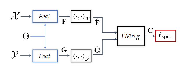
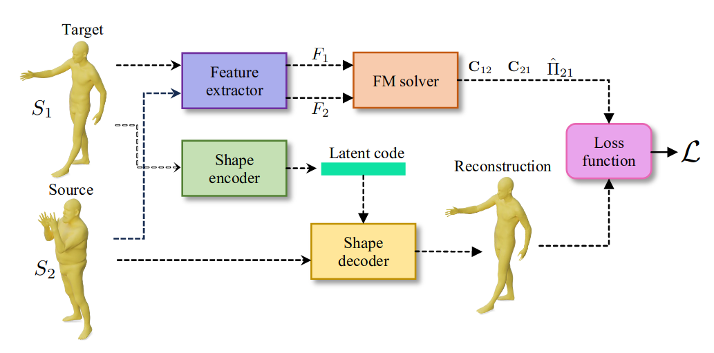
Let’s have two shapes that we wan’t to match. The natural basis functions to choose are the Laplace Beltrami Operator (LBO) eigenfunctions. Now, suppose, we know a way to define a set of functions \(f_i\) on \(N\) and \(g_j\) on \(M\) such that \(g(x) \sim f \circ T^{-1} (x)\) (local descriptors which are isometry invariant).

We decompose all \(f_i\) as \(a \in \mathbb{R}^{n \times m}\) and \(g_j\) as \(b \in \mathbb{R}^{n \times m}\). The functional map can be defined as the solution of: \[ C = \underset{C}{\text{argmin}} ||Ca - b||² \]

In practice, we compute the pointwise descriptors using a neural network. Since the output of the previous equation can be obtained in closed form, we optimize the output \(C\) with respect to the ground truth map \(C_{gt}\) or with axiomatic constraints, allowing to learn the descriptors

Functional map denoising diffusion models

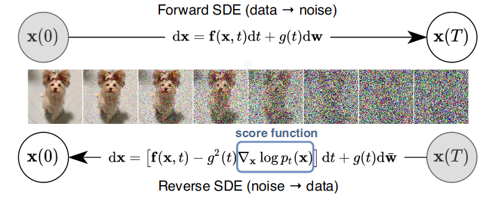
Denoising diffusion probabilistic models is currently the best way to learn a data distribution.

Starting point: learn a diffusion model on a set of already aligned non rigid shapes (for the moment, D-FAUST). We apply denoising diffusion on functional map matrices

First approach: Diffusion model as evaluator for matching

By integrating the SDE equation, we can compute the likelihood of a map. This can be used for rating quality of zero-shot matching algorithms that serves multiple potential matching outputs (Zoomout, or its evolution mapTree).

However, there is no perfect way to distinguish between right maps and maps with right orientation.

Application to point cloud matching

Zoomout only needs Laplacian decomposition to provide a match: this makes the method suitable for template to point cloud matching.

Second approach: Score distillation for functional map regularization.

We have a differentiable way of parameterizing an map \(C\) by some parameters \(\theta\) (feature extractor network). We can optimize for the quality of the map (SNK approach)

The gradient update of the parameters is given by

\[ \nabla \mathcal{L}_{\text{SDS}}(x = g(\theta)) = \mathbb{E}_{t, \epsilon} \left[ \left(\hat{\epsilon}_{\phi}(x_t, t) - \epsilon\right) \frac{dx}{d\theta}\right] \]

SNK approach

Main idea

Regularize the network with laplacian “mask” and: \[ \mathcal{L}_{\text{cycle}}, \mathcal{L}_{\text{fmap}}, \mathcal{L}_{\text{bij}}, \mathcal{L}_{\text{rec}} \]

Here, we replace \(\mathcal{L}_{\text{fmap}}\), and mask by \(\mathcal{L}_{\text{SDS}}\).

Results

Similar results when replacing \(\mathcal{L}_{\text{fmap}}\) by \(\mathcal{L}_{\text{SDS}}\). Loss of performance when removing Laplacian regularization (around 3 in geodesic error).