Non rigid diffusion:
Application to shape matching
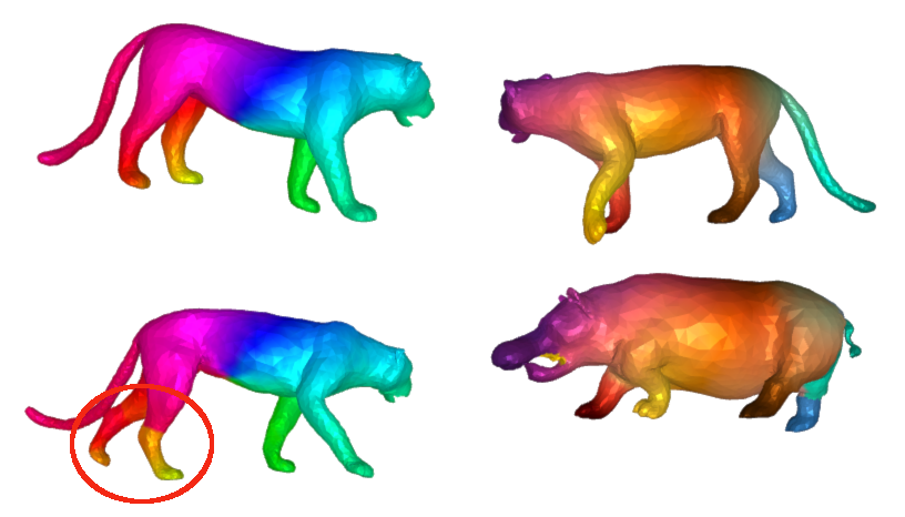
### Objective: data-driven shape matching {.smaller} ::: columns ::: {.column width="50%" .r-fit-text} Final objective: shape matching 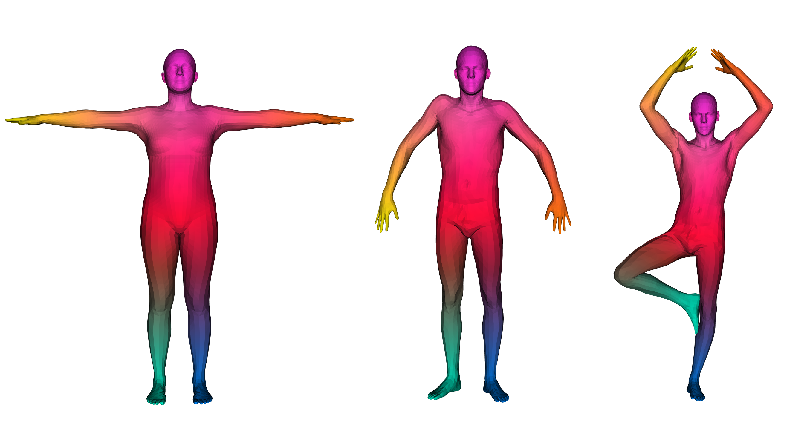 ::: ::: {.column width="50%" .r-fit-text} We have access to huge datasets of non rigid shapes nowadays. 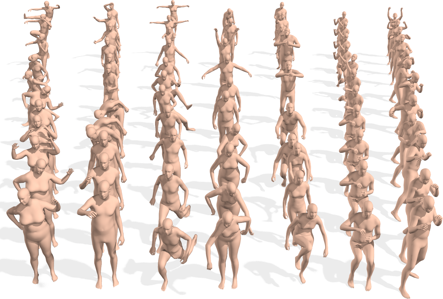 ::: ::: The objective is to take profit of some huge databases of non rigid shapes to improve shape matching algorithms. ## {.smaller} ### Shape matching algorithms are not perfect {.smaller} A general problem in non rigid shape matching is dealing with symmetries. Regularizing algorithms with axiomatic constraints are not sufficient to get rid of this problem. {.nostretch fig-align="center" width="600"} Is there a data-driven way to regularize the functional map and solve this problem ? ## Background: Functional maps {.smaller} Let $M$, $N$ two shapes. We aim to find a pointwise map $T : M \to N$ The idea is to represent the map as a map $T_F$ between function spaces $\mathcal{F}(M, \mathbb{R}) \to \mathcal{F}(N, \mathbb{R})$, such that for $f: M \to \mathbb{R}$, the corresponding function is $g = f \circ T^{-1}$. It can be shown that this map is linear. We usually represent it as a mapping matrix C between basis function (Laplace Beltrami eigenfunctions) on M and N (note: a mapping matrix $C$ does not necessarily correspond to a pointwise map). The pointwise map is then extracted from the mapping matrix. ## Background: Functional maps {.smaller .scrollable .nostretch} Let's have two shapes that we wan't to match. The natural basis functions to choose are the Laplace Beltrami Operator (LBO) eigenfunctions. Now, suppose, we know a way to define a set of functions $f_i$ on $N$ and $g_j$ on $M$ such that $g(x) \sim f \circ T^{-1} (x)$ (local descriptors which are isometry invariant). We decompose all $f_i$ as $a \in \mathbb{R}^{n \times m}$ and $g_j$ as $b \in \mathbb{R}^{n \times m}$. The functional map can be defined as the solution of: $$ C = \underset{C}{\text{argmin}} ||Ca - b||² $$ In practice, we compute the pointwise descriptors using a neural network. Since the output of the previous equation can be obtained in closed form, we optimize the output $C$ with respect to the ground truth map $C_{gt}$ or with axiomatic constraints, allowing to learn the descriptors 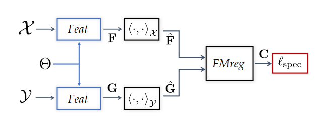{width=600} ## ### Functional map denoising diffusion models Denoising diffusion probabilistic models is currently the best way to learn a data distribution. Starting point: learn a diffusion model on a set of already aligned non rigid shapes (for the moment, D-FAUST). We apply denoising diffusion on functional map matrices 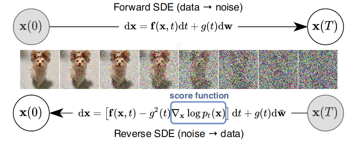 ## {.smaller} ### First approach: Diffusion model as evaluator for matching By integrating the SDE equation, we can compute the likelihood of a map. This can be used for rating quality of zero-shot matching algorithms that serves multiple potential matching outputs (Zoomout, or its evolution mapTree). However, there is no perfect way to distinguish between right maps and maps with right orientation. ## Application to point cloud matching Zoomout only needs Laplacian decomposition to provide a match: this makes the method suitable for template to point cloud matching. 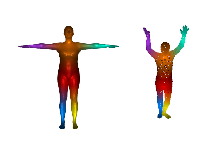 ## Second approach: Score distillation for functional map regularization. We have a differentiable way of parameterizing an map $C$ by some parameters $\theta$ (feature extractor network). We can optimize for the quality of the map (SNK approach) The gradient update of the parameters is given by $$ \nabla \mathcal{L}_{\text{SDS}}(x = g(\theta)) = \mathbb{E}_{t, \epsilon} \left[ \left(\hat{\epsilon}_{\phi}(x_t, t) - \epsilon\right) \frac{dx}{d\theta}\right] $$ ## {.smaller} ### SNK approach Main idea 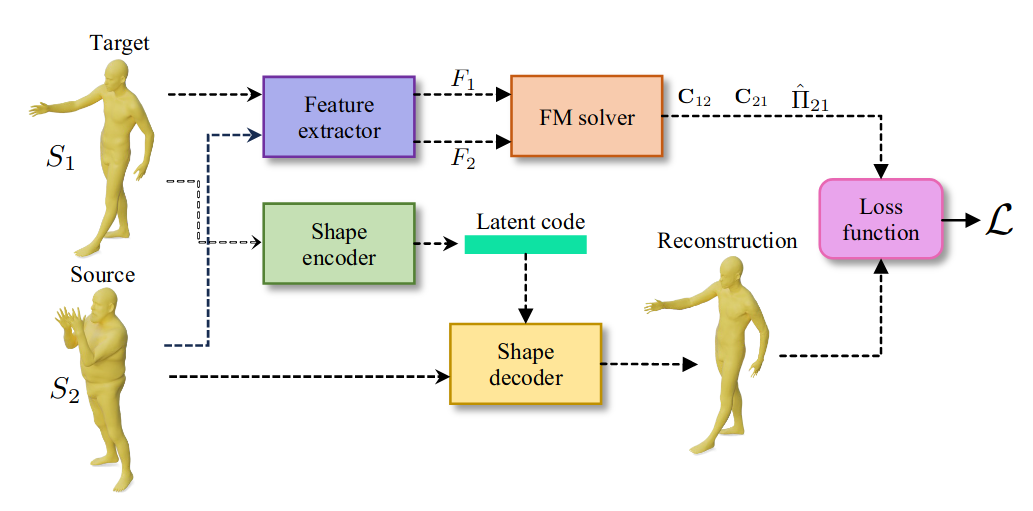 + Regularize the network with laplacian "mask" and: $$ \mathcal{L}_{\text{cycle}}, \mathcal{L}_{\text{fmap}}, \mathcal{L}_{\text{bij}}, \mathcal{L}_{\text{rec}} $$ Here, we replace $\mathcal{L}_{\text{fmap}}$, and mask by $\mathcal{L}_{\text{SDS}}$. ## Results Similar results when replacing $\mathcal{L}_{\text{fmap}}$ by $\mathcal{L}_{\text{SDS}}$. Loss of performance when removing Laplacian regularization (around 3 in geodesic error).