Denoising diffusion using Stochastic Differential Equations

LIX Seminar

Reminders: score modeling

The score function of a probability distribution with density \(p(x)\) is the gradient of the log-density: \[ \nabla_x \log p(x) \]

Working with this quantity has several advantages:

• Bypasses the normalizing constant problem
• Allows for sampling using Langevin algorithm
• It is possible to learn \(s_\theta(x) \sim \nabla_x \log p(x)\)

Evolution of the score modeling approach

Initial proposal: score matching(Hyvärinen and Dayan 2005)

The quantity \(Trace\left(\nabla_x^2 \log p_\theta(x)\right)\) is difficult to compute

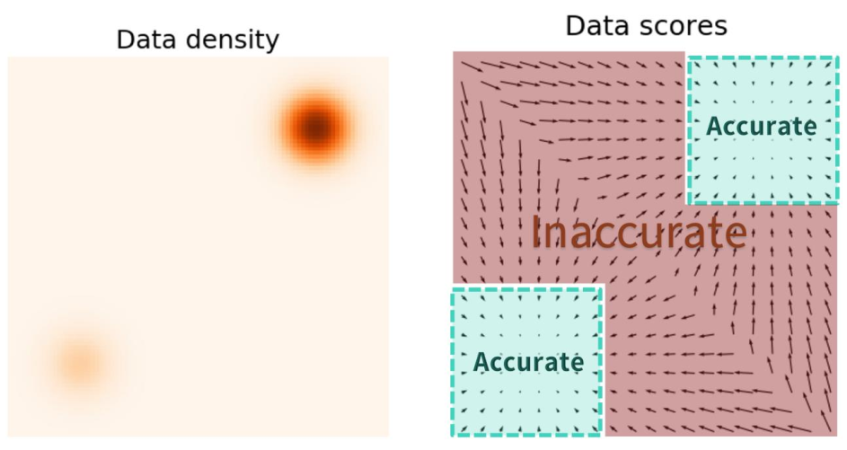
The score is untractable in low density areas

Given \(\{x_1, x_2, ..., x_T\} \sim p_\text{data}(x)\) Objective: Minimize the quantity \[ E_{p(x)}\left[\frac{1}{2}|| \log p_{\theta}(x)||² + Trace\left(\nabla_x^2 \log p_\theta(x)\right)\right]\]

 

Evolution of the score modeling approach

Initial proposal: score matching(Hyvärinen and Dayan 2005)

Learning the score of a noisy distribution(Vincent 2011)

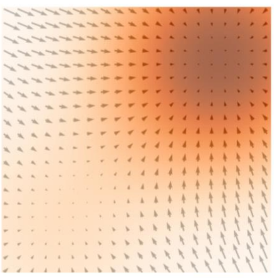
No score of noise-free distribution

Noisy distribution

Loss: \(\mathbb{E}\left[\frac{1}{2}\left|\left| s_\theta(\tilde{x})- \frac{\tilde{x}-x}{\sigma²}\right|\right|²\right]\)

Evolution of the score modeling approach

Initial proposal: score matching(Hyvärinen and Dayan 2005)

Learning the score of a noisy distribution(Vincent 2011)

Denoising diffusion models(Sohl-Dickstein et al. 2015), annealed Langevin dynamics(Y. Song and Ermon 2019)

• Gradually decrease noise in the distribution
• Can obtain non noisy samples

Annealed Langevin sampling

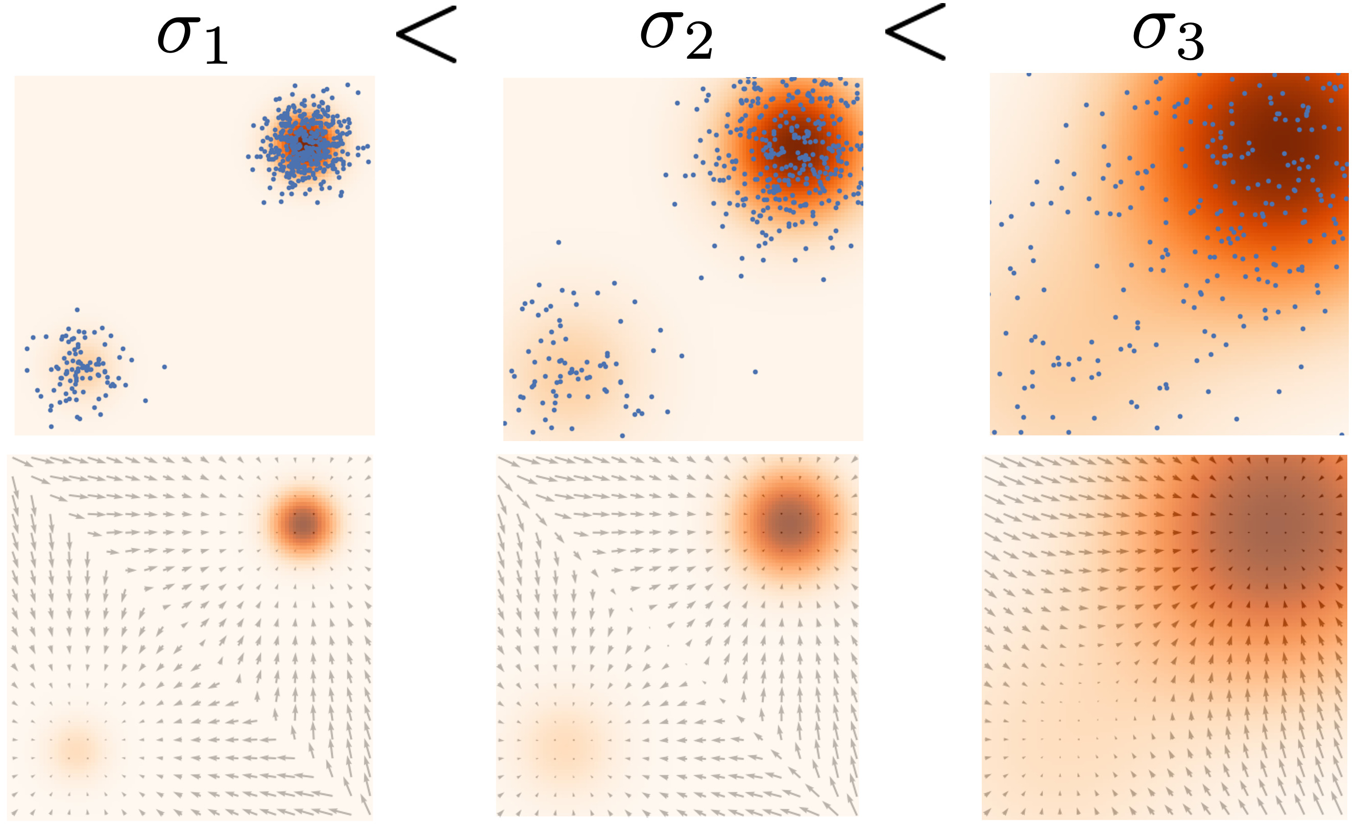
Noise conditional score model, with objective : \[ \frac{1}{L} \sum_{i=1}^L \lambda(\sigma_i) \mathbb{E}\left[\left\lvert\left\lvert s_\theta(x_i, \sigma_i) - \frac{(\tilde{x}_i - x_i)}{\sigma_i²}\right\rvert\right\rvert ² \right] \]

Evolution of the score modeling approach

Initial proposal: score matching(Hyvärinen and Dayan 2005)

Learning the score of a noisy distribution(Vincent 2011)

Denoising diffusion models(Sohl-Dickstein et al. 2015), annealed Langevin dynamics(Y. Song and Ermon 2019)

DDPM beats GAN(Ho, Jain, and Abbeel 2020)!

 

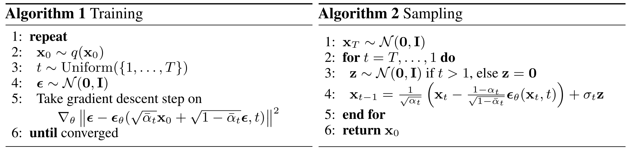
What is DDPM?

• Forward process \(x_t = \sqrt{1-\beta_t} x_{t-1} + \sqrt{\beta_t} z_t\)
• A denoiser \(\epsilon_\theta(., t)\), parameterizing the score function
• Backward process \(x_{t-1} = \frac{1}{\sqrt{1-\beta_t}} \left(x_t - \frac{\beta_t}{\sqrt{1-\alpha_t\alpha_{t-1}}}\epsilon_\theta(x_t, t)\right) + \sigma_t z_t\)
• A simple training objective \(L_\text{simple}=\left|\left|\epsilon-\epsilon_\theta\left(\underbrace{\sqrt{\bar{\alpha_t}}x_0+\sqrt{1-\bar{\alpha_t}}\epsilon}_{\text{Forward estimate of } x_t \text{ given } x_0},t\right)\right|\right|^2\)
• This objective is equivalent to the denoising score matching objective

Algorithm

 

Questions/Problems

• Can we unify DDPM and other approaches in a common framework?
• Number of timesteps \(T\) needs to be fixed before training
• Can we fasten the sampling, ideally without needed re-training?
• Can we model the data in a deterministic way using score modeling?

Proposed solution: Score modeling using Stochastic Differential Equations(Y. Song et al. 2021)!

Ordinary Differential Equations (ODE)

Equations of functions, of the form \(\frac{dx}{dt} = f(x, t)\) (order 1).

• Unique solution for any initial condition \(x(t_0)\)
• Geometric interpretation using vector fields

Stochastic diffential equations (SDE)

Equation of time-dependent stochastic processes, noted \(X_t\).

They are of the form

\(dx = \underbrace{f(x, t)dt}_{\text{"drift" term}} + \underbrace{g(t) dW_t}_{\text{"diffusion" term}}\),

where \(W_t\) is a “standard Wiener process” or Brownian motion.

They are used in many domains (finance, physics, biology, and even shape analysis)

Differences between SDE and ODE

• Given an initial condition, an SDE has now multiple possible realizations!

• The initial condition is now always \(x_0\), the time only goes Forward

• Solving an SDE means looking for the trajectories density \(p_t(x)\)

Brownian motion

A stochastic process \(W_t\) is a Wiener process, or Brownian motion, if:

• \(W_0 = 0\)
• \(W_t\) is “almost surely” continuous
• \(W_t\) has independent increments
• \(W_t - W_s \sim \mathcal{N}(0, t-s), \text{ for any } 0 \leq s \leq t\)

If we sample 100 trajectories, we obtain:

It is also the solution of the equation

\[ dx = dw \]

Properties of SDEs

Let the SDE be:

\[ dx = f(x, t)dt + g(t) d\bar{w} \]

• Assuming some conditions on \(f(x, t)\) and \(g(t)\), the density \(p_t(x)\) at any time step is uniquely determined

• Suppose we know, the score \(\nabla_x \log p_t(x)\) for all \(t\), then we can reverse the diffusion SDE using the following reverse-SDE:

\[ dx = \left[f(x,t) - g(t)² \nabla_x \log p_t(x)\right] dt + g(t) d\bar{w}, \]

where the time is flowing backwards, and \(\bar{w}\) is a backward Wiener process.

Illustration with images

Generate data from noise by reversing the perturbation procedure.

Forward and backward SDEs illustated

Reverse SDE/Annealed Langevin Dynamics

The Langevin dynamics uses the following updates:

\[ x_{t+1} \leftarrow x_t + \epsilon s_\theta (x, t) + \sqrt{2\epsilon} z_t \]

Which is similar to the reverse SDE (\(f(x, t)= 0\)): \[ dx = - g(t)² \nabla_x \log p_t(x) dt + g(t) d\bar{w}, \]

“Variance Exploding” SDE

This formulation is equivalent to denoising score matching of (Y. Song and Ermon 2019). We perturb the data by adding noise \(\tilde{x}_i \sim \mathcal{N}(x, \sigma_i² I)\). The forward process is such that

\[ x_i = x_{i-1} + \sqrt{\sigma_i² - \sigma_{i-1}²}z_{i-1}, z_{i-1} \sim \mathcal{N}(0, I) \]

Seen as the discretization of a continuous process, it becomes:

\[ \begin{align} x(t + \Delta t) & = x(t) + \sqrt{\sigma²(t+\Delta t) - \sigma²(t)} z(t) \\ & \simeq x(t) + \sqrt{\frac{d\left[\sigma²(t)\right]}{dt} \Delta t} z(t) \end{align} \]

The SDE formulates as \[ dx = \sqrt{\frac{d\left[\sigma²(t)\right]}{dt}} dw \]

“Variance preserving” SDE

This formulation is equivalent to the DDPM paper. The forward process of DDPM is given by:

\[ x_i = \sqrt{1-\beta_i} x_{i-1} + \sqrt{\beta_i} z_i = \sqrt{1-\frac{\bar{\beta}_i}{N}} x_{i-1} + \sqrt{\frac{\bar{\beta}_i}{N}} z_i \]

Where \(\bar{\beta_i} = N \beta_i\).

Seen as the discretization of a continuous process, it becomes:

\[ \begin{align} x(t + \Delta t) & = \sqrt{1-\beta(t+\Delta t) \Delta t}x(t) + \sqrt{\beta(t+\Delta t) \Delta t} z(t) \\ & \simeq x(t) - \frac{1}{2} \beta(t+\Delta t) \Delta t x(t) + \sqrt{\beta(t+\Delta t) \Delta t} z(t) \text{ (Taylor expansion) } \\ & \simeq x(t) - \frac{1}{2} \beta(t) \Delta t x(t) + \sqrt{\beta(t) \Delta t} z(t) \end{align} \]

The SDE formulates as \[ dx = - \frac{1}{2} \beta(t) x dt + \sqrt{\beta(t)}dw \]

Comparisons of behavior of both SDEs

With original data distribution -> two diracs

 

The variance exploding SDE has more curvature when approaching data \(\to\) DDPM obtains better samples with fewer steps.

Note: other samplers, such as DDIM(J. Song, Meng, and Ermon 2020) or EDM(Karras et al. 2022) can show even better curvature

Comparison to discrete approach

Training:

• The timesteps are now sampled in a continuous way
• No change in the loss

At test time:

• Possibility to use black-box SDE solvers (reduces timesteps)
• Or use generalization of annealed Langevin (denoising + correction step)

Results

Results

256x256 bedroom images (LSUN dataset)

1024x1024 face images (FFHQ dataset)

Probability flow ODE

Another remarkable result: Given the following SDE:

\[ dx = f(x, t)dt + g(t) d\bar{w}, \]

the following ODE :

\[ dx = \left[f(x, t) - \frac{1}{2}g(t)² \nabla_x \log p_t(x)\right] dt, \]

share the same marginals \(p_t(x)\) as the SDE solution, if \(p_0\) or \(p_T\) is given(Maoutsa, Reich, and Opper 2020).

In the case of the 1D brownian motion, we have

\[ \nabla_x \log p_t(x) = \frac{d}{dx}\left(-\frac{1}{2} \frac{x²}{t}\right) = -\frac{x}{t} \]

The ODE is:

\[ \frac{dx}{dt} = \frac{x}{2t}; \text{ so } x(t) = \alpha \sqrt{t} \]

Advantages of the ODE

Uniqueness: a data sample \(x(0)\) has a unique “latent” corresponding point \(x(T)\).

• First consequence: “latent” manipulation of images

Note : We can’t manipulate the latents in a differentiable way. You would need a different approach, such as score distillation sampling(Poole et al. 2022) or ControlNet(Zhang, Rao, and Agrawala 2023)

• Second consequence: the choice of the model doesn’t matter

Advantages of the ODE

We can use well established solvers. It reduces the number of evaluation steps

Samples of images, with different number of network evaluations

Compared to stochastic sampling, it reduces the number of needed evaluations from \(\mathcal{O}(d)\) to \(\mathcal{O}(\sqrt{d})\), where \(d\) is the dimension of the data(Chen et al. 2023).

Summary

Controllable generation (inverse problems)

Let \(y\), an image generated from a system \(f(x) = y\).

We can estimate the score of \(p(x | y)\):

\[ \begin{align} \nabla_x \log p_t(x(t)|y) &\simeq \nabla_x \log \int p_t(x(t)|y(t))p(y(t) |y)dy \\ & \simeq \nabla_x \log p_t(x(t)|\hat{y}(t)) ;\ \ \ \ \hat{y}(t) \sim p(y(t)|y) \\ & = \log p_t(x(t)) + \nabla_x \log p_t(\hat{y}(t)|) \\ & \simeq s_\theta(x(t), t) + \nabla_x \log p_t(\hat{y}(t)| x(t)) \end{align} \]

If the distribution \(p_t(\hat{y}(t)| x(t)))\) is tractable, we can solve the inverse problem

Controllable generation examples

Colorizing gray images using controllable generation

Inpaiting of images using controllable generation

Summary

Findings of the paper:

• Most approach of score modeling can be unified in a common framework, including DDPM
• This framework allows for better sample quality and Higher resolution for images
• The ODE formulation allows for latent encoding and high sampling speed, without needing retraining

Potential follow-up works

• Better SDE, training and even faster sampling : EDM(Karras et al. 2022)
• Differentiable image generation (for text to 3D): Score Distillation Sampling(Poole et al. 2022)
• Controllable image generation : ControlNet(Zhang, Rao, and Agrawala 2023)

References

Chen, Sitan, Sinho Chewi, Holden Lee, Yuanzhi Li, Jianfeng Lu, and Adil Salim. 2023. “The Probability Flow ODE Is Provably Fast.” In Thirty-Seventh Conference on Neural Information Processing Systems. https://openreview.net/forum?id=KD6MFeWSAd.

Ho, Jonathan, Ajay Jain, and Pieter Abbeel. 2020. “Denoising Diffusion Probabilistic Models.” Advances in Neural Information Processing Systems 33: 6840–51.

Hyvärinen, Aapo, and Peter Dayan. 2005. “Estimation of Non-Normalized Statistical Models by Score Matching.” Journal of Machine Learning Research 6 (4).

Karras, Tero, Miika Aittala, Timo Aila, and Samuli Laine. 2022. “Elucidating the Design Space of Diffusion-Based Generative Models.” In Proc. NeurIPS.

Maoutsa, Dimitra, Sebastian Reich, and Manfred Opper. 2020. “Interacting Particle Solutions of Fokker–Planck Equations Through Gradient–Log–Density Estimation.” Entropy 22 (8): 802.

Poole, Ben, Ajay Jain, Jonathan T. Barron, and Ben Mildenhall. 2022. “DreamFusion: Text-to-3D Using 2D Diffusion.” arXiv.

Sohl-Dickstein, Jascha, Eric Weiss, Niru Maheswaranathan, and Surya Ganguli. 2015. “Deep Unsupervised Learning Using Nonequilibrium Thermodynamics.” In International Conference on Machine Learning, 2256–65. PMLR.

Song, Jiaming, Chenlin Meng, and Stefano Ermon. 2020. “Denoising Diffusion Implicit Models.” arXiv:2010.02502. https://arxiv.org/abs/2010.02502.

Song, Yang, and Stefano Ermon. 2019. “Generative Modeling by Estimating Gradients of the Data Distribution.” Advances in Neural Information Processing Systems 32.

Song, Yang, Jascha Sohl-Dickstein, Diederik P Kingma, Abhishek Kumar, Stefano Ermon, and Ben Poole. 2021. “Score-Based Generative Modeling Through Stochastic Differential Equations.” In International Conference on Learning Representations. https://openreview.net/forum?id=PxTIG12RRHS.

Vincent, Pascal. 2011. “A Connection Between Score Matching and Denoising Autoencoders.” Neural Computation 23 (7): 1661–74.

Zhang, Lvmin, Anyi Rao, and Maneesh Agrawala. 2023. “Adding Conditional Control to Text-to-Image Diffusion Models.”